-
- Research Article
- https://doi.org/10.99999/00000001
-
- VOL 1
- 2027
-
- Received:
- Accepted:
- Published:
Abstract
Bernstein operators provide a constructive approximation scheme whose order controls sampling density and approximation error. For quadratic and cubic monomials on the unit interval, we derive exact error polynomials from binomial factorial moments and determine their uniform maxima. The quadratic maximum occurs at the midpoint, whereas the cubic maximizer depends on the order and approaches two thirds. These identities yield explicit checks of the first-order asymptotic error and a direct procedure for selecting an operator order from a prescribed uniform tolerance. Numerical comparisons distinguish operator order from the algebraic degree of the resulting polynomial and compare analytic maxima with sampled curves. The cubic example shows why a midpoint evaluation does not determine a uniform error. Formulas, critical points, and tolerance thresholds are supplied together, providing a reproducible comparison of elementary polynomial targets within the classical theory of positive approximation operators.
Introduction
Bernstein's probabilistic proof of the Weierstrass theorem [1] introduced a constructive way to approximate continuous functions on a compact interval. Its basis functions are nonnegative and sum to one, making the operator a weighted average of sampled values. Classical treatments develop this construction within polynomial approximation and the theory of positive linear operators [2, 3, 10]. The same basis is also fundamental in geometric design, where its coefficients offer a useful description of curves [5].
A convergence theorem alone does not specify an order suitable for a given numerical tolerance. Quantitative estimates connect approximation error to smoothness, while pointwise bounds describe how the error changes across the interval [4, 9, 11]. Exact polynomial examples give a complementary perspective: every coefficient, maximum, and tolerance threshold can be calculated explicitly. They also expose distinctions between the index of an operator, the size of its sampling set, and the algebraic degree of its output.
Scope of the comparison
We consider the targets \\(q(x)=x^2\\) and \\(c(x)=x^3\\) on \\([0,1]\\). Both are convex, so their Bernstein approximants lie above the targets. Their errors vanish at the endpoints but have different interior maxima. The main identities are collected in Theorem 1; numerical consequences appear in Table 1 and Table 2. The calculation uses standard binomial moments and is intended as an explicit account of classical approximation behaviour.
The analysis proceeds from the operator definition to finite-order errors, then to order selection and asymptotic interpretation. Sampling is used to draw curves, whereas the uniform norms are determined by differentiation. This separation is essential: a visually fine grid may miss an extremum even when the plotted curve appears smooth.
Preliminaries and moment identities
The operator and its normalization
Definition 1.
For a continuous real-valued function \\(f\in C[0,1]\\) and an integer \\(n\geq1\\), the Bernstein operator of order n is defined by
The weights \\(b_{n,k}(x)=\binom{n}{k}x^k(1-x)^{n-k}\\) sum to one. If a random variable K has the binomial distribution with parameters n and x, then \\(B_n f(x)=\mathbb{E}[f(K/n)]\\). This interpretation gives positivity immediately and shows that constant and linear functions are reproduced exactly.
Notation
- Operator order
-
The integer n defining the sampling points k/n and the Bernstein basis.
- Effective degree
-
The algebraic degree after collecting coefficients in the monomial basis.
- Uniform error
-
The maximum of \\(|B_n f(x)-f(x)|\\) over the entire interval.
Factorial moments through order three
Lemma 1.
For integers \\(r\in\{0,1,2,3\}\\), the falling-factorial moment satisfies
Here \\((a)_r=a(a-1)\cdots(a-r+1)\\), with \\((a)_0=1\\). When r exceeds n, the right-hand side is zero.
Proof.
Differentiate \\((u+v)^n\\) exactly r times with respect to u, multiply by \\(u^r\\), and set \\(u=x\\), \\(v=1-x\\). For r greater than n, the derivative vanishes. This proves the identity throughout the stated range. ∎
The decompositions \\(K^2=(K)_2+K\\) and \\(K^3=(K)_3+3(K)_2+K\\) convert factorial moments to ordinary moments. Substitution into Equation (1) therefore produces the quadratic and cubic approximants without summing each binomial term separately. These elementary identities are consistent with the general moment framework for positive operators [2, 9].
Exact errors and their maxima
Finite-order identities
Theorem 1.
For every integer \\(n\geq1\\), the errors of the quadratic and cubic targets are
The quadratic uniform error is \\(1/(4n)\\). Set \\(a_n=3n-2\\). The cubic uniform error is
Proof.
Using Lemma 1, the cubic calculation can be written in the following aligned form:
The quadratic calculation follows in the same way from the second moment. Its error has derivative \\((1-2x)/n\\), so the maximum is attained at the midpoint. Both cubic factors in Equation (3) are nonnegative on the interval. Differentiating its numerator gives \\(1+2(a_n-1)x-3a_nx^2\\). The positive root is xn from Equation (4); the other root is negative. The endpoints have zero error and the positive root lies strictly between zero and one, establishing the maximum. ∎
For \\(n=1\\), the cubic approximant is the line \\(B_1c(x)=x\\), and the critical point is \\(1/\sqrt{3}\\). The formula remains valid without a separate limiting convention. As the order grows, the critical point moves towards \\(2/3\\), rather than the midpoint used in the quadratic case.
Uniform tolerance and operator order
Corollary 1.
For a prescribed tolerance \\(\varepsilon>0\\), the smallest admissible quadratic operator order is
For the cubic target, evaluating Equation (4) at successive positive integers gives the smallest order whose uniform error is at most \\(\varepsilon\\).
Proof.
The quadratic assertion is equivalent to \\(n\geq1/(4\varepsilon)\\). For the cubic error, the expansion \\(3x^2(1-x)/n+x(1-x)(1-2x)/n^2\\) tends uniformly to zero. Consequently the successive-integer procedure terminates, and its first accepted order is minimal by construction. ∎
The resulting order is a property of this sampling operator. The targets themselves already have algebraic degrees two and three, and their best polynomial approximation error is zero at those degrees. Even when n is large, the effective degrees of these Bernstein outputs remain at most two and three respectively. Polynomial invariance of this kind is also visible in the study of iterated operators [8].
Numerical comparison and reproducibility
Quadratic curves and cubic error profiles
Figure 1 compares quadratic approximants at three orders. The endpoint values are unchanged, while the largest vertical displacement occurs at one half. Increasing the order reduces that displacement in exact inverse proportion. The curves remain quadratic after coefficient collection, despite being expressed in bases with different numbers of functions.
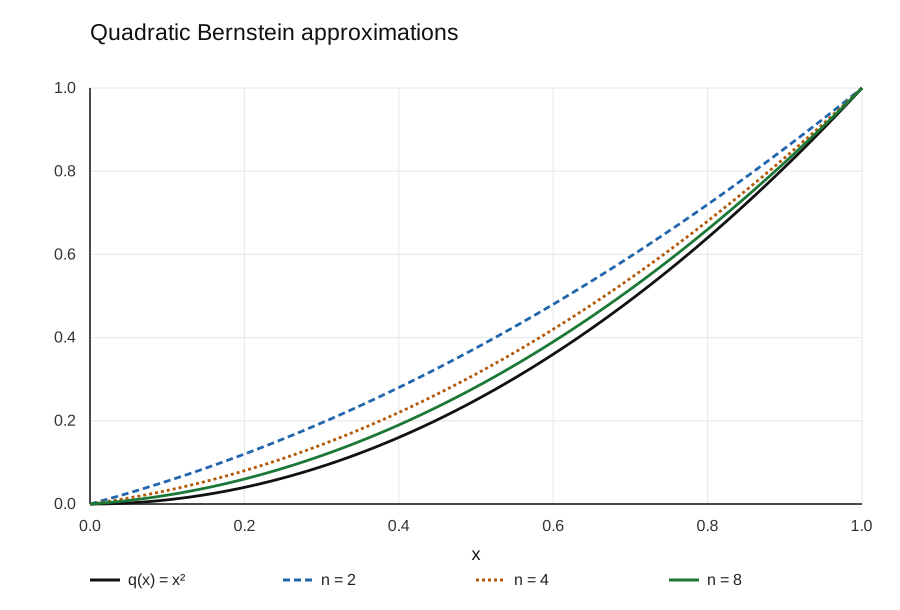
Figure 1. Quadratic target and Bernstein approximants
The target \\(q(x)=x^2\\) and its approximants \\(B_nq\\) for orders 2, 4, and 8. Each approximation meets the target at both endpoints and lies above it in the interior. The exact vertical difference is \\(x(1-x)/n\\).
The target q(x)=x^2 and its approximants B_nq for orders 2, 4, and 8. Each approximation meets the target at both endpoints and lies above it in the interior. The exact vertical difference is x(1-x)/n.
For the cubic target, multiplying the error by n makes the finite-order profiles directly comparable with their limiting shape. Figure 2 shows a peak to the right of the midpoint and a gradual movement towards two thirds. The profiles converge to \\(3x^2(1-x)\\), whose maximum is \\(4/9\\). The small correction changes both the height and location of the peak.
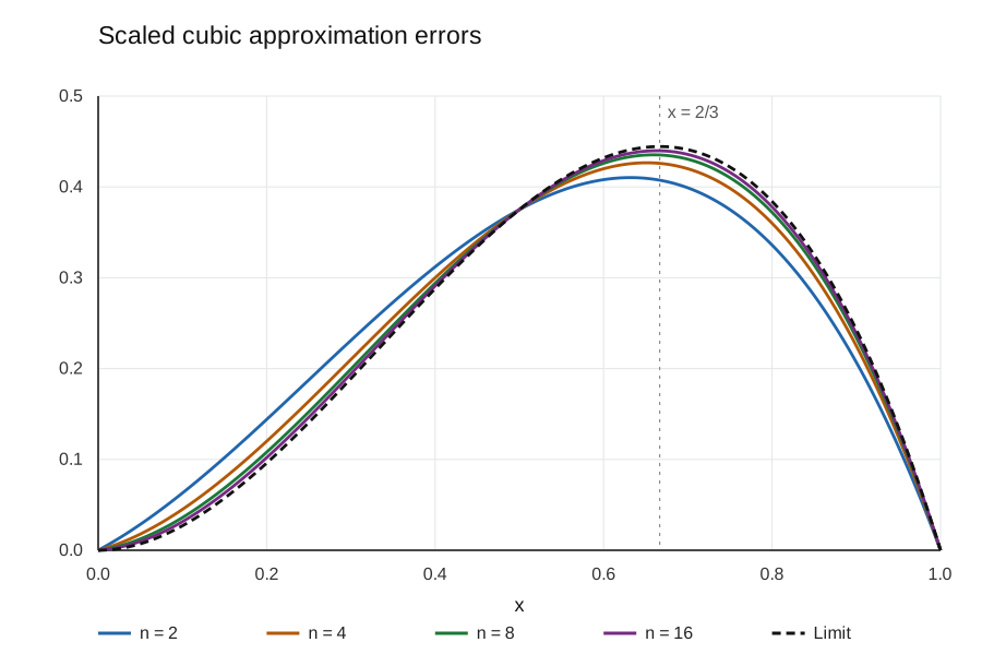
Figure 2. Scaled cubic errors and their limiting profile
Profiles \\(n(B_nc-c)\\) for orders 2, 4, 8, and 16, compared with \\(3x^2(1-x)\\). The vertical guide marks , the maximizer of the limiting profile.
Profiles n(B_nc-c) for orders 2, 4, 8, and 16, compared with 3x^2(1-x). The vertical guide marks x=23, the maximizer of the limiting profile.
Table 1 records analytic maxima rather than maxima inferred from the plotted samples. For the cubic target, the midpoint approximant equals \\(1/8+3/(8n)\\), but its midpoint error is smaller than the uniform error. Thus a single convenient evaluation point suffices only when the extremum has already been justified analytically.
Analytic values of \\(\|B_n f-f\|_\infty\\) for five operator orders. Cubic maxima are evaluated at the stationary points, with decimal values rounded to eight places.
Scroll horizontally to view full table.
| Order n | Quadratic target | Cubic target | ||
|---|---|---|---|---|
| Uniform error | Midpoint value | Uniform error | Maximizer | |
| 2 | 0.12500000 | 0.37500000 | 0.20513205 | 0.63188131 |
| 4 | 0.06250000 | 0.31250000 | 0.10664155 | 0.65118846 |
| 8 | 0.03125000 | 0.28125000 | 0.05441715 | 0.65934334 |
| 16 | 0.01562500 | 0.26562500 | 0.02749074 | 0.66310191 |
| 32 | 0.00781250 | 0.25781250 | 0.01381684 | 0.66490769 |
1 The cubic uniform error exceeds its midpoint error of 3/(8n). Both targets have zero endpoint error.
Computation protocol
The calculation follows three steps, each with a distinct purpose:
-
Reduce the binomial sums using factorial moments and retain exact rational coefficients.
-
Find every interior stationary point of the error polynomial and compare its value with both endpoints.
-
Evaluate a regular grid with spacing 0.005 for the figures and supplementary curve values.
Table 2 gives tolerance thresholds. For each accepted order, every smaller positive integer order was checked; the preceding order is also displayed in the table. Minimality follows from this complete finite check. The tolerances are absolute errors because the interval and targets have been fixed; rescaling either would change their interpretation.
The accepted order satisfies \\(\|B_n f-f\|_\infty\leq\varepsilon\\); its predecessor does not. Values are rounded to eight decimal places.
Scroll horizontally to view full table.
| Target | Tolerance | Accepted order | Error at accepted order | Error at preceding order |
|---|---|---|---|---|
| Quadratic | 0.10 | 3 | 0.08333333 | 0.12500000 |
| 0.05 | 5 | 0.05000000 | 0.06250000 | |
| 0.01 | 25 | 0.01000000 | 0.01041667 | |
| Cubic | 0.10 | 5 | 0.08600619 | 0.10664155 |
| 0.05 | 9 | 0.04848149 | 0.05441715 | |
| 0.01 | 45 | 0.00984007 | 0.01006286 |
1 Minimality was checked over all positive integers below each accepted order. These are operator orders, not minimal algebraic degrees for approximating the targets.
Independent arithmetic checks
Direct binomial summation at rational points verifies the moment-based formulas for all displayed orders. Endpoint reproduction, nonnegative errors, and polynomial degrees provide further checks. The cubic stationary-point equation is evaluated separately from the formula for the error, avoiding a circular confirmation based on the same numerical expression.
Rational point evaluations
At grid points with rational coordinates, both target values and binomial sums can be calculated as exact fractions. This removes cancellation and rounding from the identity check, while the reported critical points require square roots and are stored numerically. Supplementary Data S1 separates summary values from pointwise curve values.
Midpoint and endpoint checks
The quadratic midpoint values reduce to \\((n+1)/(4n)\\). At either endpoint, every error is zero. These checks are inexpensive and catch indexing or normalization mistakes before an extremum calculation. Appendix A gives the coefficient formulas used in the supplementary workbook.
Discussion
Relation to smoothness-based estimates
The exact errors illustrate the first-order dependence familiar from Bernstein approximation. For \\(f\in C^2[0,1]\\), the Voronovskaya asymptotic formula gives \\(n(B_nf-f)\to x(1-x)f''(x)/2\\) uniformly on the interval. For the two polynomial targets considered here, the explicit identities prove this limit directly and yield precisely the leading terms displayed above. General estimates require appropriate smoothness assumptions and are developed using moduli of smoothness [4, 9]. Strong converse inequalities connect the observed approximation rate back to smoothness [12]; two polynomial examples cannot establish those general implications.
Endpoint behaviour
Both error polynomials contain \\(x(1-x)\\), expressing exact endpoint reproduction. This factor also explains why interior and boundary behaviour differ. Pointwise estimates near the endpoints address this distinction more precisely [11]. Derivative approximation is another separate question: small function error does not by itself bound every derivative, and differentiated remainder formulas require their own analysis [6].
Limitations and alternative constructions
The comparison is restricted to noiseless polynomial targets and the classical operator. Its transparency comes from finite moment identities. For a general continuous function, the sampling values need not produce a low-degree monomial expression, and an exact maximum may be unavailable. Numerical optimization then requires appropriate certification or an explicit description of what has been sampled.
Iteration, corrected operators, and other combinations can alter the convergence rate without merely increasing the sampling order [7, 8]. Their coefficients and preservation properties must be assessed independently. The present tolerance thresholds apply only to the unmodified Bernstein sequence. They should therefore accompany the operator definition whenever reused in a computational comparison.
Three conclusions remain useful beyond these examples:
-
Operator order and algebraic degree describe different quantities.
-
The maximizer of a uniform error can depend on the order.
-
An exact error formula provides a reproducible reference for checking sampled curves.
Conclusion
Binomial factorial moments give exact quadratic and cubic Bernstein errors, including their interior maxima and tolerance-based order thresholds. The quadratic maximum is fixed at the midpoint, whereas the cubic maximum moves towards two thirds as the order increases. Reporting these analytic values alongside curve samples separates mathematical bounds from visual estimates and clarifies how the operator order controls approximation quality.
References
- [1] S. Bernstein, Démonstration du théorème de Weierstrass fondée sur le calcul des probabilités, Communications de la Société mathématique de Kharkow, deuxième série 13 (1912), no. 1, 1–2. https://www.mathnet.ru/eng/khmo107
- [2] J. Bustamante, Bernstein Operators and Their Properties, Birkhäuser, Cham, 2017. https://doi.org/10.1007/978-3-319-55402-0 https://link.springer.com/book/10.1007/978-3-319-55402-0
- [3] R. A. DeVore, G. G. Lorentz, Constructive Approximation, Springer, Berlin, Heidelberg, 1993. https://link.springer.com/book/9783540506270
- [4] Z. Ditzian, V. Totik, Moduli of Smoothness, Springer, New York, 1987. https://doi.org/10.1007/978-1-4612-4778-4 https://link.springer.com/book/10.1007/978-1-4612-4778-4
- [5] R. T. Farouki, The Bernstein polynomial basis: A centennial retrospective, Computer Aided Geometric Design 29 (2012), no. 6, 379–419. https://doi.org/10.1016/j.cagd.2012.03.001 https://www.sciencedirect.com/science/article/pii/S0167839612000192
- [6] M. S. Floater, On the convergence of derivatives of Bernstein approximation, Journal of Approximation Theory 134 (2005), no. 1, 130–135. https://doi.org/10.1016/j.jat.2004.02.009 https://www.sciencedirect.com/science/article/pii/S0021904505000523
- [7] Z. Guan, Iterated Bernstein polynomial approximations, arXiv:0909.0684v3 (preprint, 2009), version dated 16 Oct 2009. https://doi.org/10.48550/arXiv.0909.0684 https://arxiv.org/abs/0909.0684v3
- [8] R. P. Kelisky, T. J. Rivlin, Iterates of Bernstein polynomials, Pacific Journal of Mathematics 21 (1967), no. 3, 511–520. https://msp.org/pjm/1967/21-3/pjm-v21-n3-p12-s.pdf
- [9] R. Păltănea, Approximation Theory Using Positive Linear Operators, Birkhäuser, Boston, 2004. https://doi.org/10.1007/978-1-4612-2058-9 https://link.springer.com/book/10.1007/978-1-4612-2058-9
- [10] G. M. Phillips, Interpolation and Approximation by Polynomials, Springer, New York, 2003. https://doi.org/10.1007/b97417 https://link.springer.com/book/10.1007/b97417
- [11] G. Tachev, Pointwise approximation by Bernstein polynomials, Bulletin of the Australian Mathematical Society 85 (2012), no. 3, 353–358. https://doi.org/10.1017/S0004972711002838 https://www.cambridge.org/core/journals/bulletin-of-the-australian-mathematical-society/article/pointwise-approximation-by-bernstein-polynomials/1FDA2BCFB326347218DB87D0E19C6225
- [12] V. Totik, Strong converse inequalities, Journal of Approximation Theory 76 (1994), no. 3, 369–375. https://doi.org/10.1006/jath.1994.1023 https://www.math.u-szeged.hu/Bolyai/hppublikacio.phtml?id=73
Appendix
Coefficient formulas and asymptotic checks
Collecting the monomial coefficients gives
These expressions produce the pointwise supplementary values without evaluating large binomial coefficients. For the cubic target, the quadratic stationary-point equation has discriminant \\(4(a_n^2+a_n+1)\\). Selecting its positive root recovers Equation (4).
Limiting scaled errors
Multiplication by the operator order yields the exact expressions
The quadratic profile is independent of the order. The cubic correction tends uniformly to zero because \\(|x(1-x)(1-2x)|\leq1/4\\). Therefore the cubic scaled uniform error tends to \\(4/9\\), consistent with the maxima reported in the supplementary summary. No grid-based extremum estimate is needed for this limit.
Figures
Figure 1. Quadratic target and Bernstein approximants
The target \\(q(x)=x^2\\) and its approximants \\(B_nq\\) for orders 2, 4, and 8. Each approximation meets the target at both endpoints and lies above it in the interior. The exact vertical difference is \\(x(1-x)/n\\).
The target q(x)=x^2 and its approximants B_nq for orders 2, 4, and 8. Each approximation meets the target at both endpoints and lies above it in the interior. The exact vertical difference is x(1-x)/n.
Figure 2. Scaled cubic errors and their limiting profile
Profiles \\(n(B_nc-c)\\) for orders 2, 4, 8, and 16, compared with \\(3x^2(1-x)\\). The vertical guide marks , the maximizer of the limiting profile.
Profiles n(B_nc-c) for orders 2, 4, 8, and 16, compared with 3x^2(1-x). The vertical guide marks x=23, the maximizer of the limiting profile.
Tables
Analytic values of \\(\|B_n f-f\|_\infty\\) for five operator orders. Cubic maxima are evaluated at the stationary points, with decimal values rounded to eight places.
Scroll horizontally to view full table.
| Order n | Quadratic target | Cubic target | ||
|---|---|---|---|---|
| Uniform error | Midpoint value | Uniform error | Maximizer | |
| 2 | 0.12500000 | 0.37500000 | 0.20513205 | 0.63188131 |
| 4 | 0.06250000 | 0.31250000 | 0.10664155 | 0.65118846 |
| 8 | 0.03125000 | 0.28125000 | 0.05441715 | 0.65934334 |
| 16 | 0.01562500 | 0.26562500 | 0.02749074 | 0.66310191 |
| 32 | 0.00781250 | 0.25781250 | 0.01381684 | 0.66490769 |
1 The cubic uniform error exceeds its midpoint error of 3/(8n). Both targets have zero endpoint error.
The accepted order satisfies \\(\|B_n f-f\|_\infty\leq\varepsilon\\); its predecessor does not. Values are rounded to eight decimal places.
Scroll horizontally to view full table.
| Target | Tolerance | Accepted order | Error at accepted order | Error at preceding order |
|---|---|---|---|---|
| Quadratic | 0.10 | 3 | 0.08333333 | 0.12500000 |
| 0.05 | 5 | 0.05000000 | 0.06250000 | |
| 0.01 | 25 | 0.01000000 | 0.01041667 | |
| Cubic | 0.10 | 5 | 0.08600619 | 0.10664155 |
| 0.05 | 9 | 0.04848149 | 0.05441715 | |
| 0.01 | 45 | 0.00984007 | 0.01006286 |
1 Minimality was checked over all positive integers below each accepted order. These are operator orders, not minimal algebraic degrees for approximating the targets.